How to Trade Market Inefficiencies?
Trading is all about exploiting the mispricing of assets. And mispricing occurs due to market inefficiencies. So wouldn’t it be great if there was a way to identify market inefficiencies? Well, there is!
In this lesson, we’ll explore how to identify inefficiencies like trends and mean reversion using autocorrelation, and walk through a strategy to trade them. To learn more about trading such inefficiencies, check out the Quantra course on Trading Alphas: Mining, Optimisation, and System Design.

All the concepts covered in this post are taken from the Quantra course Trading Alphas: Mining, Optimisation, and System Design. You can preview the concepts taught in this post by clicking on the free preview button and going to Section 5 and Unit 1 of the course.
Note: The links in this tutorial will be accessible only after logging into quantra.quantinsti.com

Note that backtesting results do not guarantee future performance. The presented strategy results are intended solely for educational purposes and should not be interpreted as investment advice.
In this post, we will cover the following topics:
1. How to identify market inefficiencies based on autocorrelation?
2. Does timeframe matter?
3. Backtesting the Strategy
4. Performance when traded solely based on trend
5. Combining Strategies
6. Calculating Risk-Adjusted Returns
The practical implementation of the strategy is done using Python, therefore, if you’re new to Python then you’ll find the course on Python for Trading! quite helpful.
How to identify market inefficiencies based on autocorrelation?
One of the ways to spot inefficiencies in the market is by looking at autocorrelation, which tells us whether the past returns of an asset can help predict its future returns.
Positive autocorrelation signals that past returns tend to predict future returns, meaning trends are likely to continue. On the flip side, negative autocorrelation suggests that prices revert to their mean after deviating—a behaviour known as mean reversion. Recognising these patterns can help you design strategies that leverage market inefficiencies. Let’s plot a slope to get an understanding of the relationship between the past and current returns of SPY.
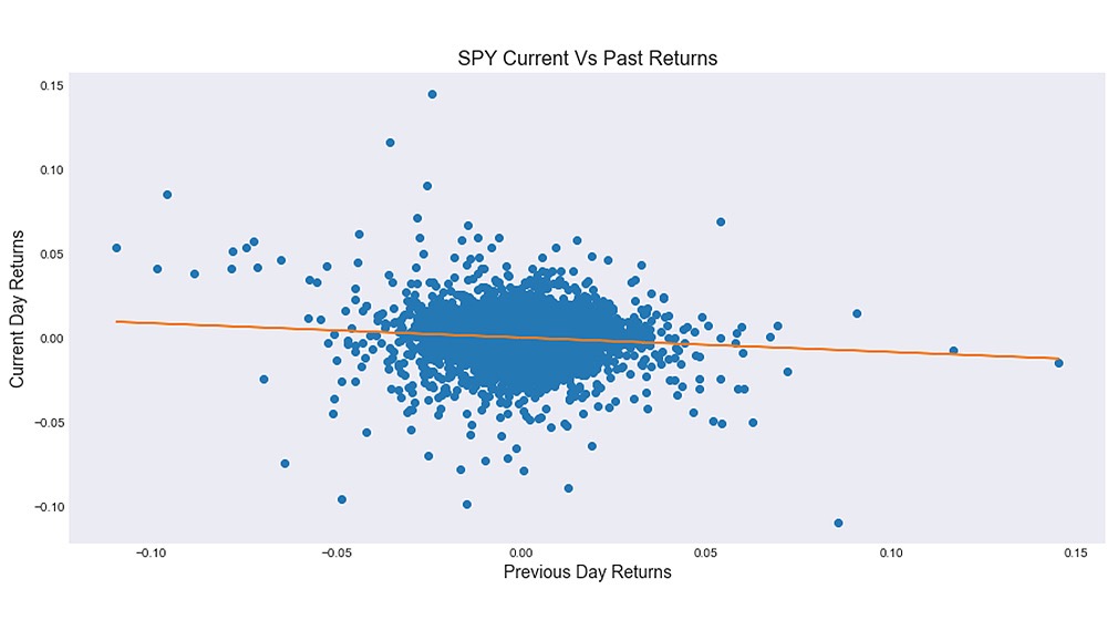
As you can see, we have a downward-sloping line. This leads us to the conclusion that in this timeframe, the SPY returns must be mean-reverting. This means whenever SPY strays away from its average price, it tends to bounce back. So, if the previous day’s returns are negative, there’s a higher likelihood the next day’s returns will be positive.
Does timeframe matter?
It’s important to note that market inefficiencies can vary depending on the timeframe. While daily data might reveal mean-reverting properties, a longer timeframe might highlight trends. For instance, in the case of SPY, we may see mean reversion on a daily basis, but when we zoom out to 3-month data, the same asset might show a clear trend. Understanding this shift is crucial for building a robust trading strategy.
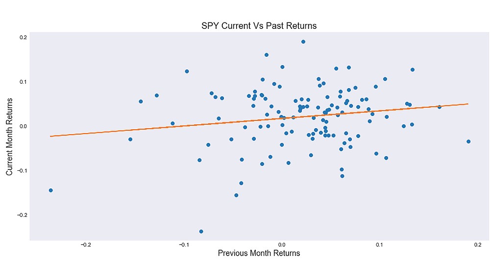
As you can see, the downward-sloping line (as seen earlier with daily data) is now sloping upwards when we zoom out to 3-month data. This means trends are likely to continue.
Backtesting the Strategy
We are already using the returns data of SPY which depicts the percentage change in price from one point to another. To backtest the strategy, we’ll simply multiply the sign of the previous day’s return by the current day’s return. In the case of 3-month data we will multiply the sign of the previous 3-month return by the current 3-month return.
This allows us to determine how autocorrelation impacts returns. For example, in the case of trending series (positive autocorrelation) if the previous 3-month return is negative, we expect the current 3-month return to follow suit. Based on this, we take trades—so we will get positive returns when the signs match, and negative returns when they don’t.
Example 1:
Previous Day Return = -1
Current Day Return = 2
Since the previous day’s return was negative, we expected another negative return and took a short position. However, the current return was positive. The signs don’t match, so the strategy return or the return generated on this trade is negative: (-1 x 2 = -2).
Example 2:
Previous Day Return = -1
Current Day Return = -2
Here, the negative previous day’s return led us to expect a negative return again. A short position was taken, and the actual return was negative, as expected. The signs match, resulting in a positive strategy return: (-1 x -2 = 2).
This method allows us to assess how well the strategy performs based on autocorrelation expectations.
Performance when traded solely based on trend
Let’s backtest the strategy using 3-month data, where we observed positive autocorrelation and thus placed trades based on trends.
To evaluate the performance of this strategy, we'll analyse the correlation between the strategy returns and the benchmark returns. Similar to our previous analysis of SPY's current and past returns, we’ll plot the slope—this time, for the strategy’s returns versus the market's.
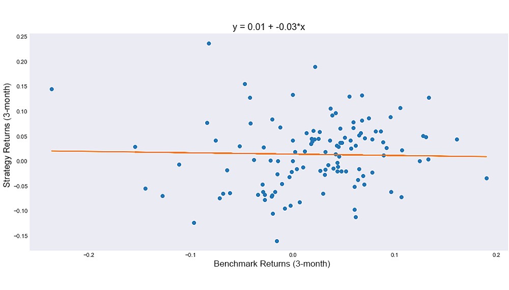
The equation ???? = 0.01 + −0.03*???? represents a linear regression model where:
???? denotes the strategy returns (dependent variable)
???? denotes the benchmark returns (independent variable)
0.01 is the intercept (also called the alpha)
-0.03 is the slope (which represents beta, or how sensitive the strategy is to the benchmark).
As you can see, the correlation is close to 0 and the alpha is 0.01 on a quarterly basis, which gives us an annualised alpha of 4% per year (1 x 4).
Not too impressive. How can we improve this strategy?
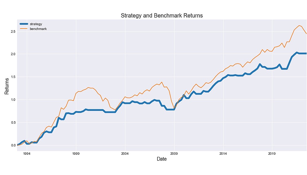
Combining Strategies
Let’s try combining a buy-and-hold strategy for SPY with a three-month momentum strategy. First, we’ll add the returns of both strategies and divide the sum by two, as we’re allocating resources equally between them.
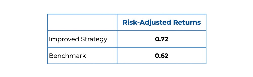
Calculating Risk-Adjusted Returns
Risk-adjusted returns measure how much return you’re generating for every dollar of risk. To calculate this, divide the mean return by the standard deviation of returns, then multiply by the square root of the periods in a year. In this case, we have 4 quarters, so the square root is 2.
In this post, we backtested multiple strategies, which can easily be done using Python. Want to learn how you can do it too? You can learn more about the implementation of this strategy in Python by accessing Section 5, Unit 1 of the course.

About the Author:
The course "Trading Alphas: Mining, Optimisation, and System Design" was co-authored by Dr. Thomas Starke, CEO of AAAQuants, an Australia-based prop-trading and consultancy firm for automated trading systems. Dr Starke has authored 3 patents, and 20+ peer-reviewed research papers with over 400 citations. He has also been a presenter at over 100 international conferences. Check out more courses by Dr. Thomas Starke here.
IMPORTANT DISCLAIMER: This post is for educational purposes only and is not a solicitation or recommendation to buy or sell any securities. Investing in financial markets involves risks and you should seek the advice of a licensed financial advisor before making any investment decisions. Your investment decisions are solely your responsibility. The information provided is based on publicly available data and our own analysis, and we do not guarantee its accuracy or completeness. By no means is this communication sent as the licensed equity analysts or financial advisors and it should not be construed as professional advice or a recommendation to buy or sell any securities or any other kind of asset