How to Use Machine Learning in Trading?
Did you know that machine learning algorithms can add value to your trading strategies or investment portfolio?
Machine learning is like having a financial Sherlock Holmes on your team, sifting through heaps of historical data to uncover hidden patterns and practical insights. The ML model doesn't just stop at pointing out trading opportunities but also suggests exit points and fine-tuning trade sizes.
In this post, we will look at the step-by-step process of creating and backtesting a machine learning-based trading system. If you are new to machine learning, Python for Machine Learning course would be helpful.
Note that backtesting results do not guarantee future performance. The presented strategy results are intended solely for educational purposes and should not be interpreted as investment advice.
All the concepts covered in this tutorial are taken from the Quantra course on Python for Machine Learning in Finance. You can preview the concepts taught in this course by clicking on the free preview button.
Note: The links in this tutorial will be accessible only after logging into quantra.quantinsti.com


The following topics are covered in this Quantra Classroom:
- The Need for Machine Learning in Trading
- Real-World Applications of Machine Learning in Trading
- Anatomy of a Machine Learning-Based Trading System
- Backtesting
- Analysing performance
The Need for Machine Learning in Trading
The need for machine learning in trading has grown significantly in recent years, as financial markets have become increasingly complex and competitive.
Machine learning techniques offer a powerful tool for traders and financial institutions to make sense of vast amounts of data, detect patterns, and make informed decisions in real-time. These algorithms can analyse historical market data, news sentiment, and a wide array of economic indicators to identify potential trading opportunities and manage risks more effectively.
As markets become more data-driven and sophisticated, the integration of machine learning in trading is no longer a luxury but a necessity for those seeking a competitive edge.
Real-World Applications of Machine Learning in Trading
One of the most prominent applications of machine learning is algorithmic trading, where machine learning models are employed to automate the execution of trades, optimising strategies, and responding to market changes at lightning speed.
Sentiment analysis, another crucial application, leverages natural language processing to process news articles, social media, and other textual data to gauge market sentiment and make informed trading decisions.
Risk management is also greatly enhanced through machine learning, as predictive models can assess and mitigate potential risks in real-time. Machine learning has undoubtedly become a cornerstone of modern trading, providing invaluable insights, risk mitigation, and efficiency in a dynamic and data-rich financial landscape.
Anatomy of a Machine Learning-Based Trading System
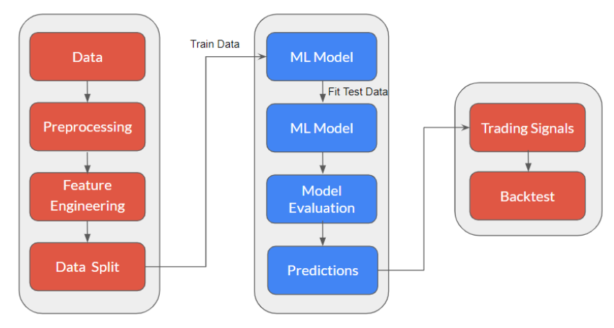
Figure: Anatomy of Machine Learning Model
This is a general structure for using machine learning for trading. It involves the following steps:
- Data Collection
- Data Preprocessing
- Feature Engineering
- Data Split
- Train Model with Training Data
- Fit Test Data on Model
- Evaluate the Model
Continuous monitoring and optimisation are essential to keep the system adaptive and profitable in evolving market conditions.
Let’s try to make this classroom interesting. In this classroom, you will try to answer the problem statement, “Should you buy JP Morgan stock or not?”
You will need some data before you decide to buy or sell JP Morgan. This leads us to the first step.
Step 1: Data Collection
You can gather historical market data, such as stock prices, volume, and relevant economic indicators.
How do you collect data?
You should access data from trusted sources or APIs, ensuring data quality and accuracy.
Let’s take JP Morgan’s price data from January 3, 2017 to December 31, 2019.
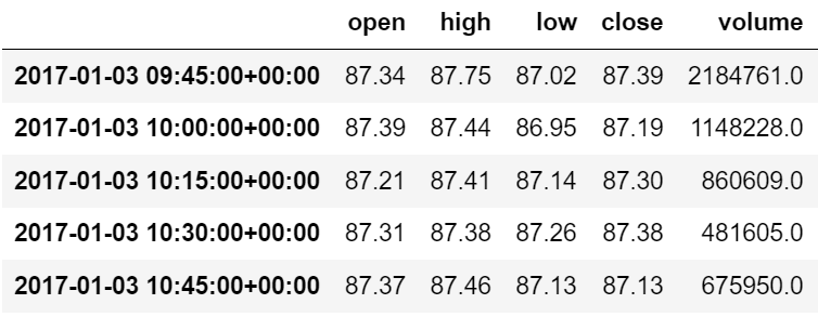
Figure: JP Morgan’s OHLCV Data
This is the 15-minute price and volume data of JP Morgan, which includes the Open, High, Low, and Close prices along with the Volume data.
Step 2: Data Preprocessing
Before you input the data into the machine learning model, you should make sure that the data is correct.
For example, in the table below, from 10:45 to 11:00 am, the close price was $87. But from 11:15 to 11:30 am it was recorded as $890. This means that there is some error in the data.
Also, from 11:30 to 11:45 am, the close price was 0, which seems odd.
|
Date-Time |
Close |
|
2024-03-04 10:45:00-11:00:00 |
$87 |
|
2024-03-04 11:00:00-11:15:00 |
$890 |
|
2024-03-04 11:15:00-11:30:00 |
$89 |
|
2024-03-04 11:30:00-11:45:00 |
$0 |
These are a few things you should check before using the data further. There are various functions in Python which handle all pre-processing tasks efficiently.
Step 3: Feature Engineering
Before we started talking about the machine learning model, we had put a question, “Should you buy JP Morgan or not?”
A simple answer to this would be, “If I am sure that JP Morgan will increase in the next 15 minutes or next time period, then I will buy.”
This means we are trying to predict whether the stock price will move up or not in the next 15 minutes or next time period.
Let’s introduce the concept of the target variable here. The target variable is what the machine learning model tries to predict to solve the problem statement. It is referred to as y.
How to create the target variable?
We will create a column, target. First, we will calculate the percentage change of the close prices. If the percentage change is positive, we will make the target variable as 1, otherwise 0. Since we are creating a model to predict future price movements, we will also shift the target variable by 1 time period.
Thus, the target column will have two labels, 1 and 0. Whenever the label is 1, the model indicates a buy signal. And whenever the label is 0, the model indicates do not buy.
Let’s say on January 3, from 10 am to 10:15 am, if the close price moves up, then you will keep the target variable as 1 for January 3, from 9:45 to 10 am.
You can learn more about the target variable by watching the video in the course Python for Machine Learning in Finance

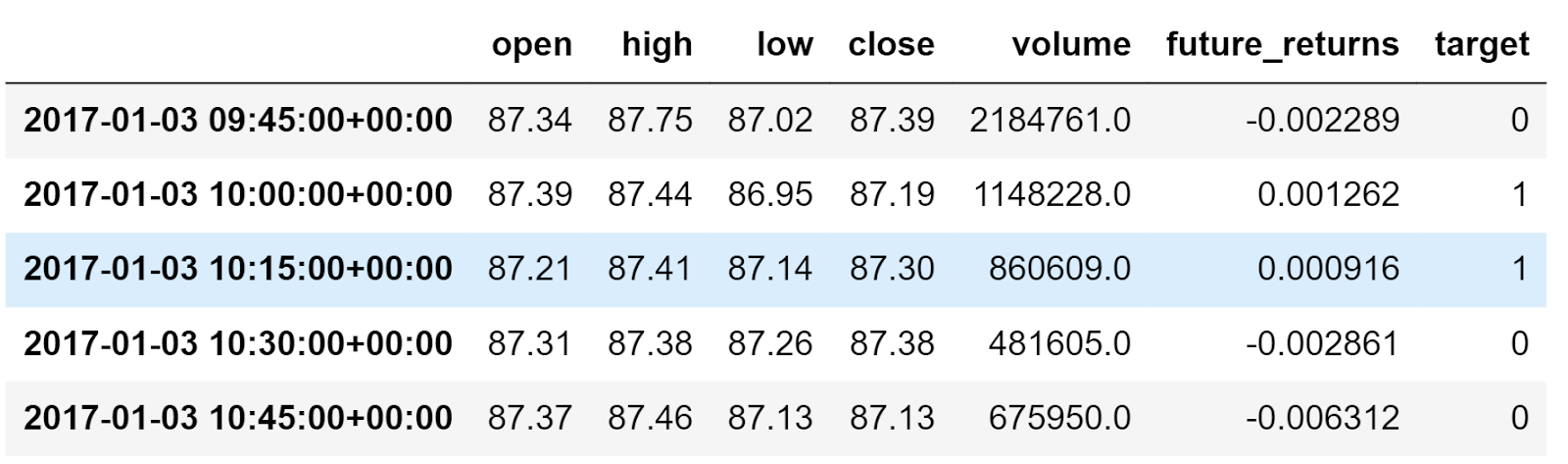
Figure: Target Variable
Now comes the interesting part. In order to predict the signal, you will create the input variables for the ML model. These input variables are called features. It is referred to as X. You can create features on the basis of:
- Percentage change in the last n time periods: 1-period, 2-period.
- Technical indicators: RSI, ADX
- Volatility and other parameters.
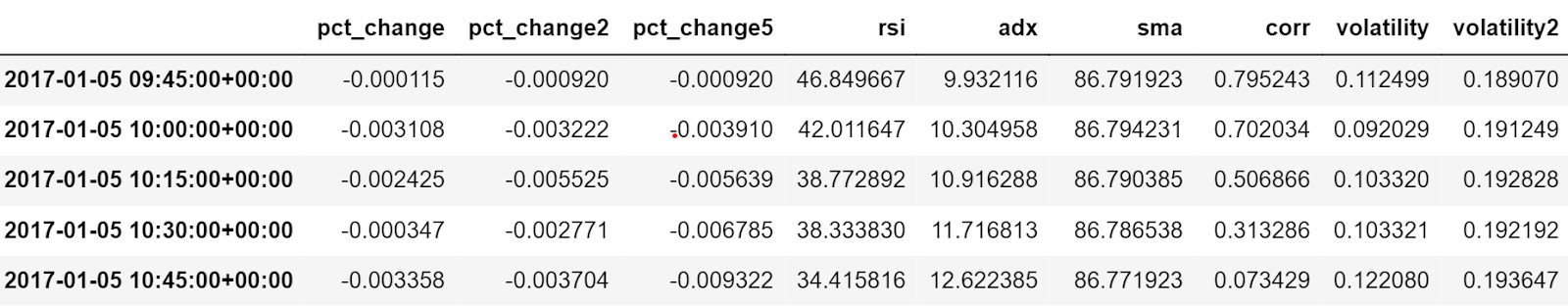
Figure: Input Features
Step 4: Data Split
Before you can apply machine learning to a trading strategy, you have to train the model first. This is similar to learning about a certain topic and then taking an exam on it.
But a machine learning model expects features to be stationary so that it can learn properly. Thus, you would apply a technique called scaling. Here, you will scale the input features in a certain range. There are different methods available, such as Min-Max scaling, Normalisation etc.
After scaling, the features would look something like this.
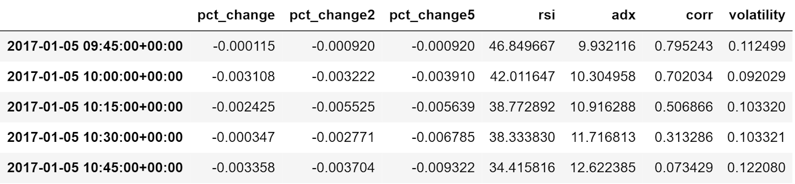
Figure: Scaled Data
Now that our data is scaled, we will split the data.
In our case, you will split the X and y datasets in the ratio 80:20 for “train” and “test”. This means that you will use 80% of your data to train the model and then 20% for testing the model on how well the model learned.
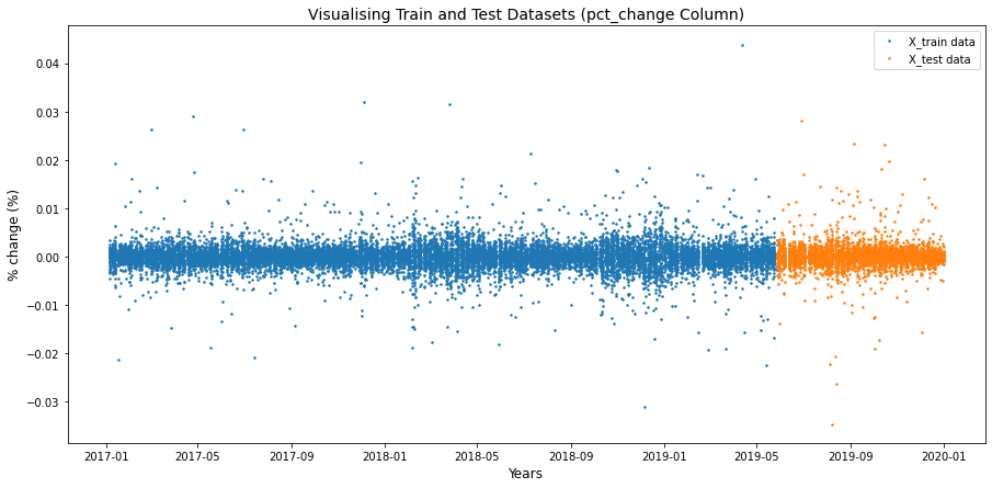
Figure: Visualisation of Train and Test
You can see that the dataset is from 2017 to 2019. 80% of the dataset, i.e. from January 2017 to 28 May 2019 is in the train dataset, X_train and the rest of the dataset is in the test dataset X_test.
Step 5: Train Model with Training Data
Choose a machine learning algorithm such as a decision tree, random forest, or neural network. Train the model using the training dataset, optimising hyperparameters as necessary.
For this classroom, you will use the Random Forest Classifier model.
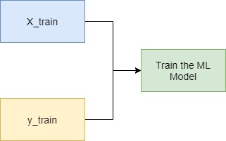
Figure: Train the ML Model
In essence, it will check the features for a given time period and will try to understand which values will give the target variable as buy, which is represented by 1.
Step 6: Fit Test Data on Model
Once the model is trained, you use the trained model to make predictions on the test dataset. Remember that when we split the dataset, the test dataset was from the date June 1, 2019 to December 31, 2019.
Now, it will check the input feature values in the test dataset and try to predict whether the stock will move up or not. This prediction will be saved in the column “y_pred”.
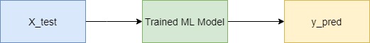
Figure: Predict on Test Data
Step 7: Evaluate the Model
Assess model performance using various metrics like accuracy, precision, recall, and F1-score for the model.
Accuracy is basically checking how many times was the model right in predicting the correct class. For example, if the model correctly predicts the target variable 90 out of 100 times, then the model’s accuracy is 90%. Similarly, there are other measures to help us understand the model’s performance.
Backtesting
Once, you are confident that your model is reasonably good at predicting whether JP Morgan should be bought or not, you will deploy the model to make real-time predictions based on current market data.
Interpret model predictions to generate buy, sell, or hold signals.
Here, if the model predicts that the stock price would move up in the next time period, we buy the stock. If the model predicts that the stock price will not move up, then we take no position, or sell the stock if we have already bought the stock.
Further, we will implement risk management rules, such as setting stop-loss and take-profit levels.
Finally, you will simulate the trading strategy using historical data to assess its performance over time. Calculate returns, drawdowns, and other relevant statistics. Make adjustments to the strategy based on backtesting results.
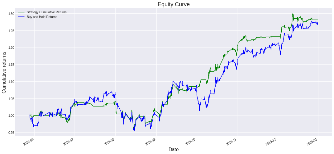
Figure: Strategy returns of machine learning-based trading strategy
Following a backtesting analysis conducted on JP Morgan's stock price spanning from June 2019 to January 2020, the cumulative returns of this strategy amounted to 1.28 times the initial investment. This translates to a CAGR of 52%. It is important to note that backtesting results do not guarantee future performance. The presented strategy results are intended solely for educational purposes and should not be interpreted as investment advice. A comprehensive strategy evaluation across multiple parameters is necessary to assess its effectiveness.
It is important to note that backtesting results do not guarantee future performance. The presented strategy results are intended solely for educational purposes and should not be interpreted as investment advice. A comprehensive evaluation of the strategy across multiple parameters is necessary to assess its effectiveness.
The creation of target and feature variables presented in the classroom has been covered in detail, along with the Python code in this unit.

What to do next?
- Go to this course
- Click on 'Free Preview'
- Go through 10-15% of course content
- Drop us your comments and queries on the community
IMPORTANT DISCLAIMER: This email is for educational purposes only and is not a solicitation or recommendation to buy or sell any securities. Investing in financial markets involves risks and you should seek the advice of a licensed financial advisor before making any investment decisions. Your investment decisions are solely your responsibility. The information provided is based on publicly available data and our own analysis, and we do not guarantee its accuracy or completeness. By no means is this communication sent as the licensed equity analysts or financial advisors and it should not be construed as professional advice or a recommendation to buy or sell any securities or any other kind of asset.