Creating a Cross-Sectional Mean Reversion Strategy
In the context of time series mean reversion, we think of it as a stock’s prices reverting to a mean determined by its own historical prices.
But is it possible to create a long-short portfolio of multiple stocks by applying the mean reversion logic? The answer is yes!
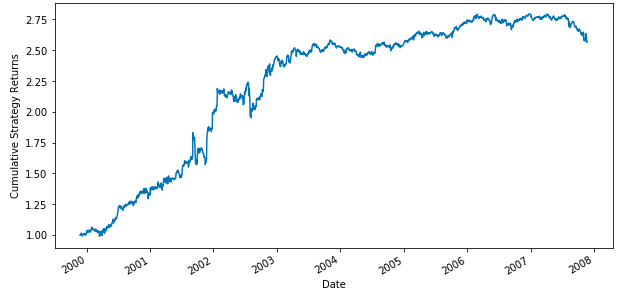
In this post, you will learn how to build a long-short portfolio based on cross-sectional mean reversion. We tested this strategy on a portfolio of multiple assets and these were the results:
It is important to note that backtesting results do not guarantee future performance. The presented strategy results are intended solely for educational purposes and should not be interpreted as investment advice. A comprehensive evaluation of the strategy across multiple parameters is necessary to assess its effectiveness.
All the concepts covered in this post are taken from the Quantra course on Mean Reversion Strategies in Python. You can preview the concepts taught in this course by clicking on the free preview button and going to Section 14 and Unit 1 of the course.
Note: The links in this tutorial will be accessible only after logging into quantra.quantinsti.com

What is Cross-Sectional Mean Reversion?
As mentioned earlier, when we think of time series mean reversion, we take it as prices reverting to a mean determined by their own historical prices. But today, our spotlight is on the Long-Short portfolio strategy, a game-changer relying on cross-sectional mean reversion.
Here's the thing – in cross-sectional mean reversion, we're not just eyeing the absolute returns of stocks; we're also getting into the short-term relative returns. Think about this – if Apple outperforms Google today, the expectation is that Google will have its day in the sun tomorrow. It's all about the underperformance leading to overperformance, and vice versa.
Building the Long-Short Portfolio
Now, let's roll up our sleeves and talk about constructing this Long-Short portfolio. The beauty of this strategy is that it doesn't hinge on long-term stationarity or cointegration of stocks. Instead, it's all about ranking stocks based on some criterion. Let's say, for example, we use the 1-day return as our criterion.
Here's the play-by-play:
- Ranking Stocks: We rank stocks based on our chosen criterion – in this case, the 1-day return.
- Buying and Shorting: We buy the stocks with the worst previous day returns and short the ones with the best returns. It's a daily dance of rebalancing the portfolio.
- Capital Allocation: The burning question – how do we divide up our capital among these stocks? It's linearly proportional to the average return of the portfolio minus the return of the stock on that day. In other words, if a stock has a very high positive return relative to its peers, we will short more of that stock. On the other hand, if it has a very high negative return relative to its peers, we will buy lots of it. Essentially, we're betting more on underperformers and less on overperformers.
Walk Through of the Strategy
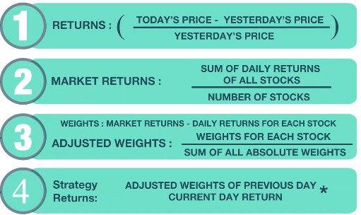
Let's break down the process:
- Calculate Daily Returns: Subtract today’s price from yesterday’s price, and divide by yesterday's price.
- Calculate Average Market Returns: Sum daily returns for all stocks, divided by the number of stocks.
- Calculate Weights: Subtract market returns from daily returns of Apple.
- Adjusted Weights: Adjust weights by dividing Apple’s weight by the sum of all absolute weights.
- Capital Allocation: Positive or negative weights dictate going long or short. Zero weight means no position.
- Calculate Strategy Returns: Multiply the adjusted weight of the previous day with the return of the stock for the current day.
The steps mentioned can be summarised as follows:
The Performance
The cumulative strategy returns graph shows the performance of the cross-sectional mean reversion strategy on a portfolio consisting of multiple assets stocks:
This strategy has generated an annualised strategy return of 12.44% and a Sharpe Ratio of 1.04x. It is important to note that backtesting results do not guarantee future performance. The presented strategy results are intended solely for educational purposes and should not be interpreted as investment advice. A comprehensive evaluation of the strategy across multiple parameters is necessary to assess its effectiveness.
Conclusion
To sum up, we've learned how the concept of mean reversion can be applied to create a long-short portfolio. By focusing on short-term relative returns, this approach takes advantage of a pattern of ups and downs.
You can also learn more about the implementation of the cross-sectional mean reversion strategy using Python. All you have to do is take a free preview of Section 14 Unit 4 of the “Mean Reversion Strategies In Python” course on Quantra.
What to do next?
- Go to this course
- Click on
- Go through 10-15% of course content

Drop us your comments and queries on the community
IMPORTANT DISCLAIMER: This post is for educational purposes only and is not a solicitation or recommendation to buy or sell any securities. Investing in financial markets involves risks and you should seek the advice of a licensed financial advisor before making any investment decisions. Your investment decisions are solely your responsibility. The information provided is based on publicly available data and our own analysis, and we do not guarantee its accuracy or completeness. By no means is this communication sent as the licensed equity analysts or financial advisors and it should not be construed as professional advice or a recommendation to buy or sell any securities or any other kind of asset.