TStatistics

Introduction

A t-statistic or test statistic is a standardised value calculated from sample data during a hypothesis test. Its purpose is to help determine whether to reject or accept a null hypothesis. The distribution of these t-statistics is known as the student t distribution.

 

According to an old rule of thumb, when the sample size is below 30 (small sample size), it is more appropriate to use the t statistic and the t distribution table to find the probability of the sample data lying within or outside a critical sample parameter.

Over a period of time, the appropriateness of using the t-statistics depends on the specific situation of the data. Some of these situations include:

 

• Population Standard Deviation: If the population standard deviation is unknown and needs to be estimated from the sample, the t-statistics is often used. In contrast, when the population standard deviation is known, the z-statistic (based on the standard normal distribution) can be employed.

 

• Normality Assumption: The t-statistics assumes that the data follows a normal distribution. If the data significantly deviates from normality, the t-test's validity may be compromised. In such cases, non-parametric tests may be more appropriate.

 

• Independence of Observations: The t-test assumes that the observations in the sample are independent of each other. Violation of this assumption may lead to inaccurate results.

 

• Type of Hypothesis Test: The t-statistics is commonly used for hypothesis testing involving means, such as the comparison of means between two groups (independent samples t-test) or within the same group at different times (paired samples t-test).

 

• Known Population Parameters: In situations where the population parameters are precisely known, other statistical tests or confidence interval estimation methods may be more appropriate than the t-test.

 

• Outliers and Skewness: Extreme outliers or significant skewness in the data can influence the t-test results. Robust statistical methods may be used to handle such situations.

 

---

 

Formula of t-statistics

The formula for the t-statistics is given as:

t = (x - μ) / (s / sqrt(n))

 

Where,                

x is the sample mean

μ is the population mean

s is the standard deviation of the sample

n is the sample size

 

---

 

Example

Let's illustrate this with an example:

ABC manufactures light bulbs, and the CEO claims that on average, a light bulb lasts 300 days with a standard deviation of 50 days. To investigate the claim, we want to find the probability that 15 randomly selected bulbs would have an average life of no more than 290 days.

Since the sample size (n = 15) is less than 30, we will use the t distribution.

 

Given: μ = 300, s = 50, and n = 15.

 

We can calculate the t-statistics as follows:

t = (290 - 300) / (50 / sqrt(15)) = -0.774

 

Next, we determine the degrees of freedom (df) as n - 1, which gives us 14.

 

Now, we want to find P(X <= 290), which is equivalent to finding P(t <= -0.774). 

Referring to the t distribution table with 14 degrees of freedom, we directly find the cumulative probability value for t = -0.774, which is 0.226. 

 

Therefore, the probability that a randomly selected light bulb will last less than 290 days is 0.226.

 

If the question asked for the probability of the average life being more than 290 days (P(X >= 290)), we would calculate it as P(t >= -0.7745966) = 1 - P(t <= -0.7745966) = 0.774.

 

---

 

Degrees of freedom and t- statistics

To compute a probability from the table, we need two values: 

• Degrees of freedom and the 
• T statistic

 

The degrees of freedom represent the number of independent observations in the data set. 

It tells you how much flexibility or variability you have when dealing with data. The more degrees of freedom you have, the more options you have to "move around" or make changes without breaking the rules or assumptions of the analysis.

For example, if you only have one stock to invest in, your degrees of freedom are limited. You have just one choice to make, and that's it. On the other hand, if you have multiple stocks to choose from and can allocate your money between them, you have more degrees of freedom. You can decide how much money to put into each stock, and you have more flexibility in shaping your investment portfolio.

 

---

 

Advantage of degrees of freedom in trading

Having more degrees of freedom in trading can be advantageous because it allows you to diversify your investments, reduce risk, and potentially increase your overall returns. It's like having more options to manoeuvre and adapt your strategy based on market conditions and your risk tolerance.

 

However, keep in mind that too many degrees of freedom can also lead to analysis paralysis or over-trading. It's essential to strike a balance and make informed decisions based on sound research and analysis rather than making impulsive moves with all the options available to you.

 

When estimating a mean score or proportion from a single sample, the number of independent observations is equal to the sample size minus one.

For instance, if the sample size is 8, the degrees of freedom would be 8 - 1 = 7.

 

---

 

Formulas for Degrees of freedom (df) in different hypothesis tests

Degrees of freedom (df) in hypothesis tests refer to the number of independent pieces of information that are available to estimate the parameters of a statistical model. 

 

The formula for degrees of freedom varies depending on the type of hypothesis test being conducted. 

 

Let's explore the formulas for different types of hypothesis tests:

One-Sample T-Test

The one-sample t-test is used to determine whether the mean of a single sample differs significantly from a known or hypothesised population mean. 

 

The formula for degrees of freedom in a one-sample t-test is:

df = n - 1

where "n" is the sample size.

 

Independent Samples T-Test: 

The independent samples t-test is used to compare the means of two independent groups (samples) to determine if there is a significant difference between them. 

 

The formula for degrees of freedom in an independent samples t-test is:

df = (n1 + n2) - 2

where "n1" is the sample size of the first group and "n2" is the sample size of the second group.

 

Paired Samples T-Test: 

The paired samples t-test (also known as the dependent samples t-test) is used when you have two sets of data that are related or paired in some way, and you want to determine if there is a significant difference between their means. 

 

The formula for degrees of freedom in a paired samples t-test is:

df = n - 1

where "n" is the number of pairs or observations in the data.

 

In each of these scenarios, the degrees of freedom play a crucial role in determining the appropriate critical values from t-distributions and, consequently, the p-values associated with the hypothesis tests.

 

---

 

Using T-statistics in trading

Using t-statistics in trading can provide traders with a statistical edge and help them make more informed decisions. T-statistics play a crucial role in hypothesis testing, confidence interval estimation, and risk management, which are all essential aspects of successful trading strategies. 

 

Here's how traders can effectively use t-statistics in their trading activities:

 

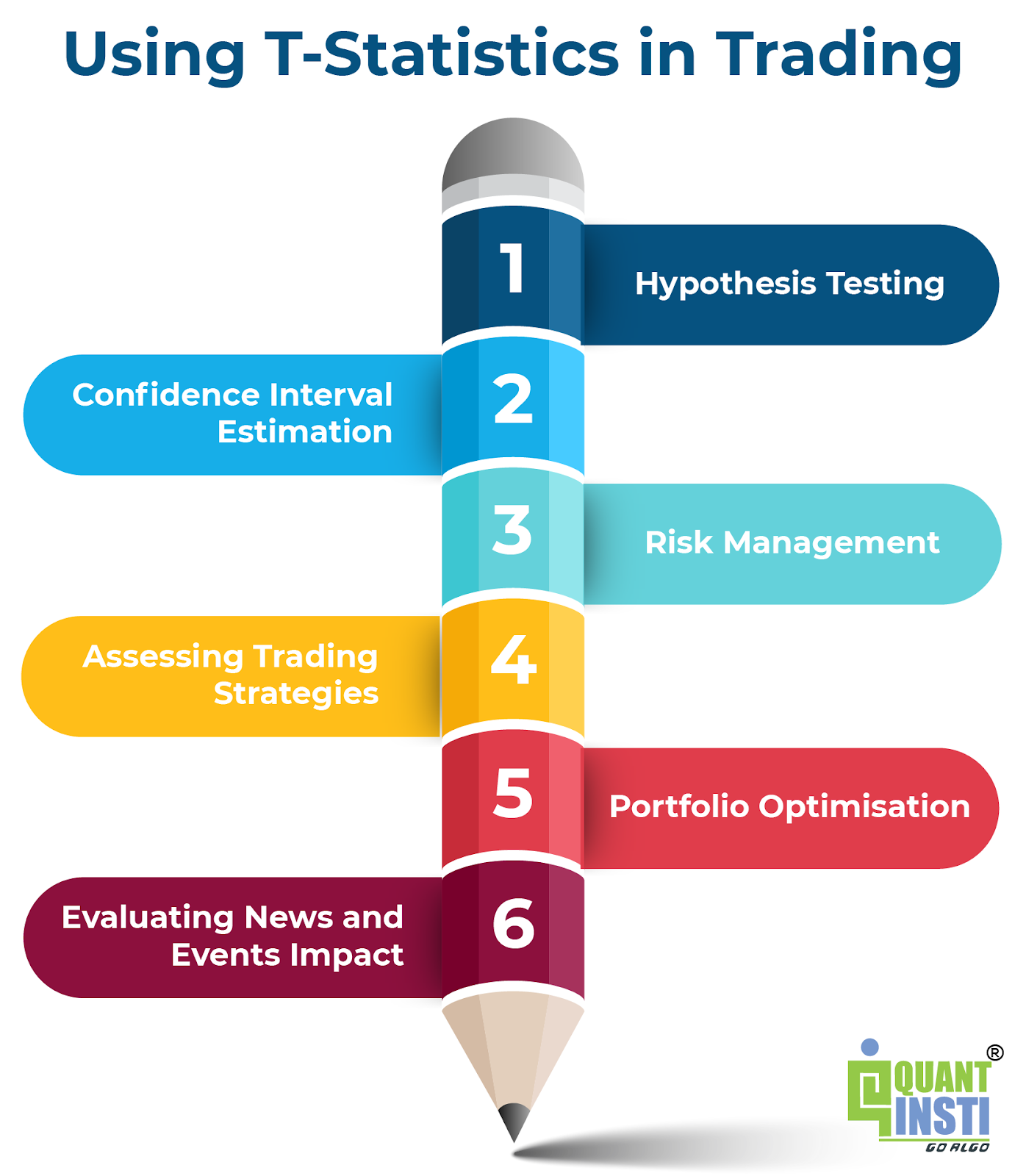
1. Hypothesis Testing:

Traders can use t-statistics for hypothesis testing to validate or refute trading strategies or market assumptions. For example, a trader might have a hypothesis that a particular technical indicator can predict stock price movements. By collecting historical data and calculating the t-statistics for the indicator's performance, the trader can determine whether the indicator's average return is significantly different from zero (i.e., whether it has predictive power).

 

2. Confidence Interval Estimation:

Traders often use confidence intervals to estimate the range of potential outcomes for key trading parameters, such as expected returns or volatility. The t-distribution table helps traders determine critical t-values for constructing these intervals based on a desired level of confidence. For example, traders can calculate the confidence interval for a stock's expected return and use it to assess potential risks and rewards.

 

3. Risk Management:

T-statistics can be utilised in risk management to estimate Value at Risk (VaR), which quantifies the maximum potential loss a trader can expect at a specific confidence level over a given time horizon. By calculating the t-statistics and finding the critical t-value for the chosen confidence level, traders can determine the VaR and implement appropriate risk management strategies to protect their capital.

 

4. Assessing Trading Strategies:

T-statistics can be applied to evaluate the performance of trading strategies and determine their statistical significance. When comparing the returns of a trading strategy to a benchmark or alternative approach, traders can calculate the t-statistics to ascertain if the strategy's outperformance (or underperformance) is statistically significant or merely due to chance.

 

5. Portfolio Optimisation:

In portfolio optimisation, traders can use t-statistics to assess the statistical significance of correlations between assets. A high positive t-statistics indicates a strong positive correlation, which may influence portfolio diversification decisions. Conversely, a low t-statistics suggests a weak correlation, indicating potential benefits from adding the asset to the portfolio to reduce overall risk.

 

6. Evaluating News and Events Impact:

When assessing the impact of news or events on asset prices, t-statistics can help determine whether the observed price movements are statistically significant or merely random noise. By calculating the t-statistics for returns around a specific event and comparing it to the critical t-value, traders can gauge the event's significance on market behaviour.